Uni-variate & Distributional Analysis
Summary of the Dataset
| Age |
49.09 |
50.00 |
18.17 |
18 |
34.00 |
50.00 |
65.00 |
80.00 |
80.00 |
| Tenure |
34.68 |
34.00 |
21.04 |
0 |
16.00 |
34.00 |
52.25 |
72.00 |
72.00 |
| MonthlyCharges |
68.51 |
69.02 |
29.07 |
18 |
43.74 |
69.02 |
92.65 |
119.77 |
119.77 |
| TotalCharges |
2339.68 |
1900.12 |
1808.26 |
0 |
938.64 |
1900.12 |
3380.87 |
8444.03 |
8444.03 |
Random 10 samples from the dataset
| Male |
21 |
14 |
No |
Fiber optic |
One year |
26.52 |
371.28 |
No |
| Female |
25 |
64 |
Yes |
DSL |
One year |
24.08 |
1541.12 |
No |
| Female |
20 |
8 |
No |
None |
Month-to-month |
106.34 |
850.72 |
No |
| Male |
80 |
68 |
No |
Fiber optic |
One year |
100.87 |
6859.16 |
No |
| Female |
26 |
24 |
No |
DSL |
Month-to-month |
87.13 |
2091.12 |
Yes |
| Female |
52 |
7 |
No |
None |
One year |
18.00 |
126.00 |
No |
| Male |
64 |
34 |
Yes |
None |
Two years |
86.90 |
2954.60 |
No |
| Female |
40 |
30 |
No |
None |
Month-to-month |
74.62 |
2238.60 |
Yes |
| Male |
42 |
5 |
Yes |
DSL |
Month-to-month |
79.93 |
399.65 |
No |
| Male |
74 |
24 |
No |
Fiber optic |
Two years |
113.12 |
2714.88 |
No |
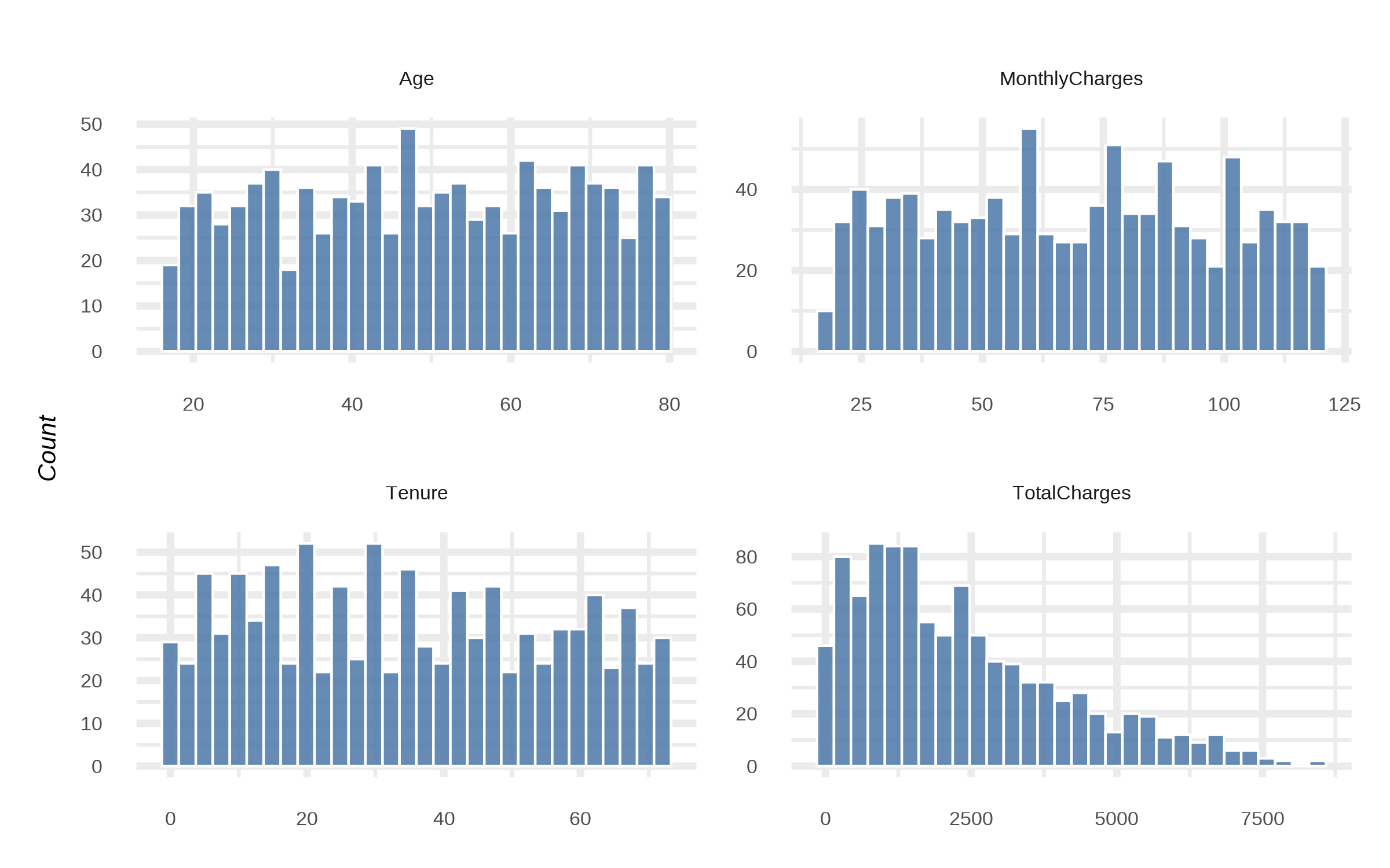
Numeric Distributions (Histograms)
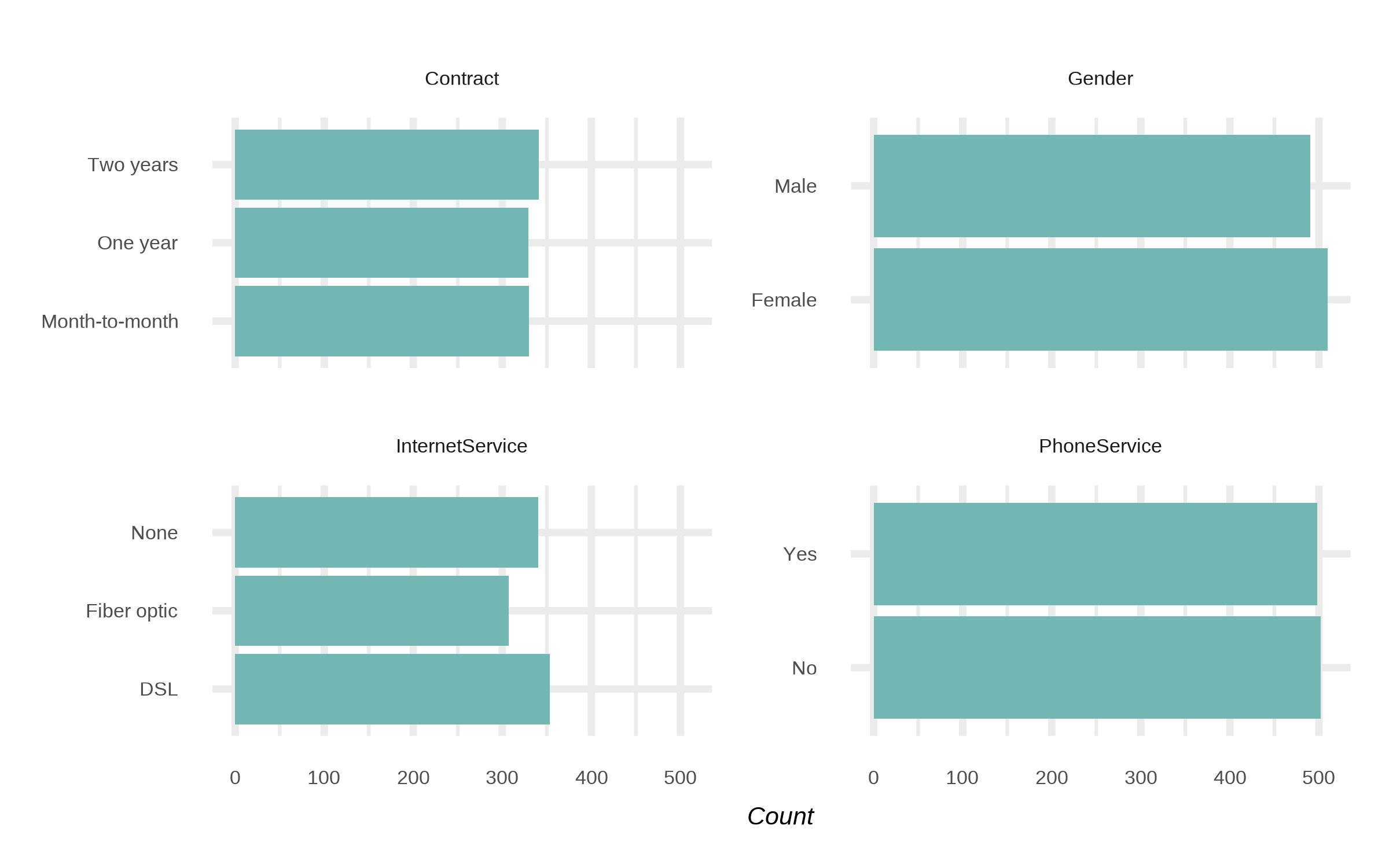
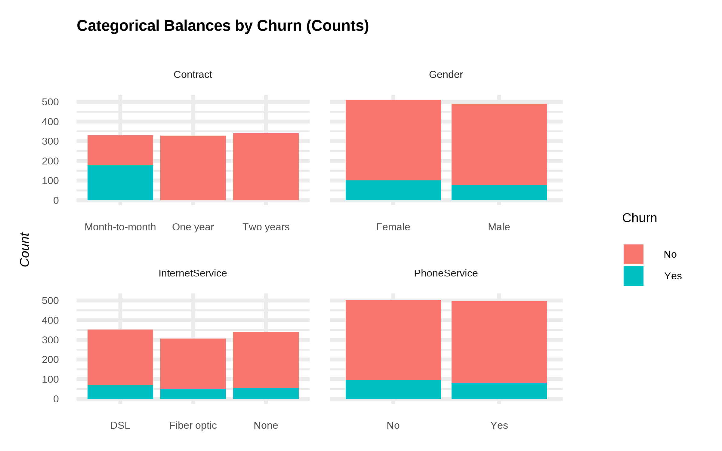
Categorical Counts (Phone/Internet/Contract)
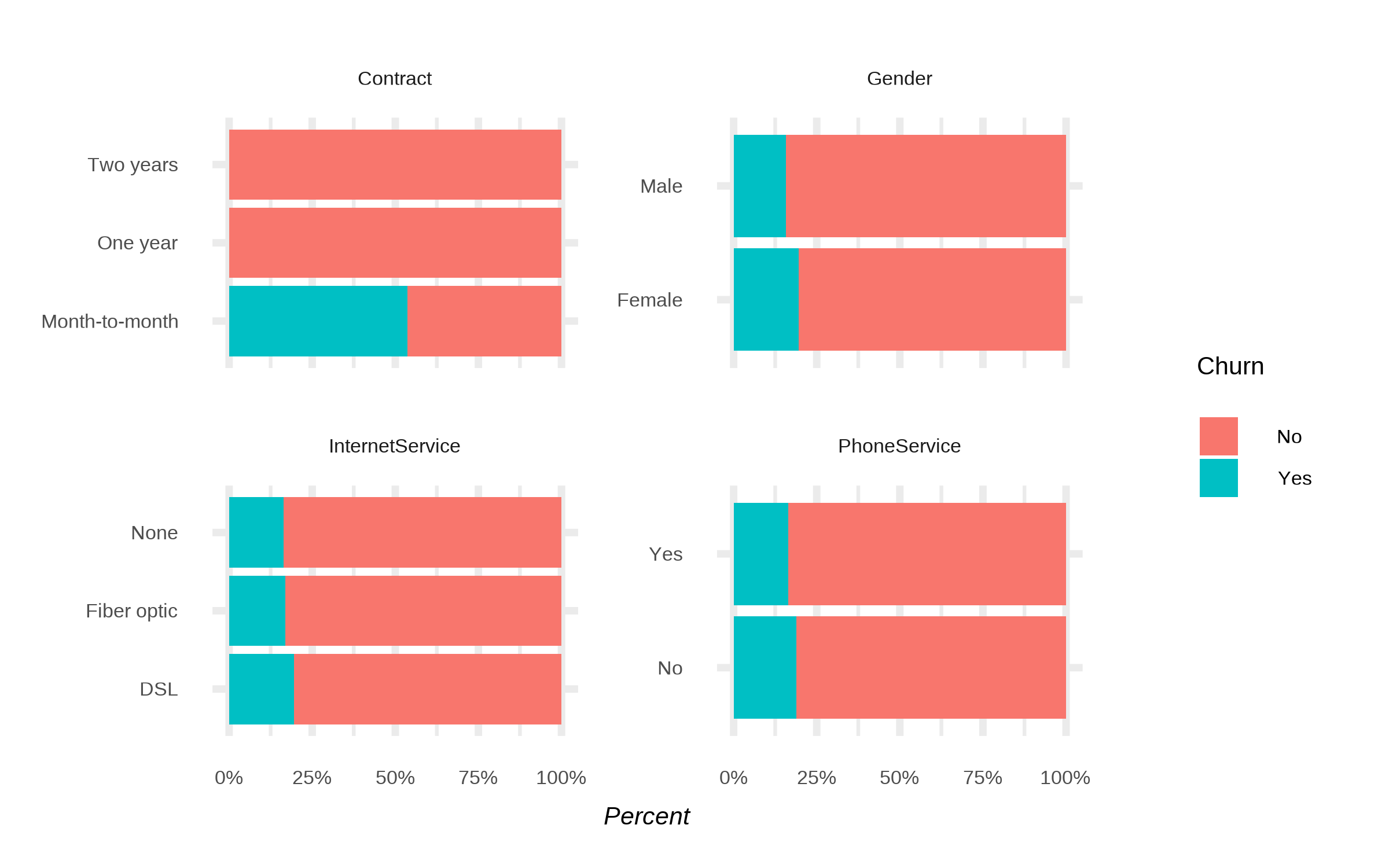
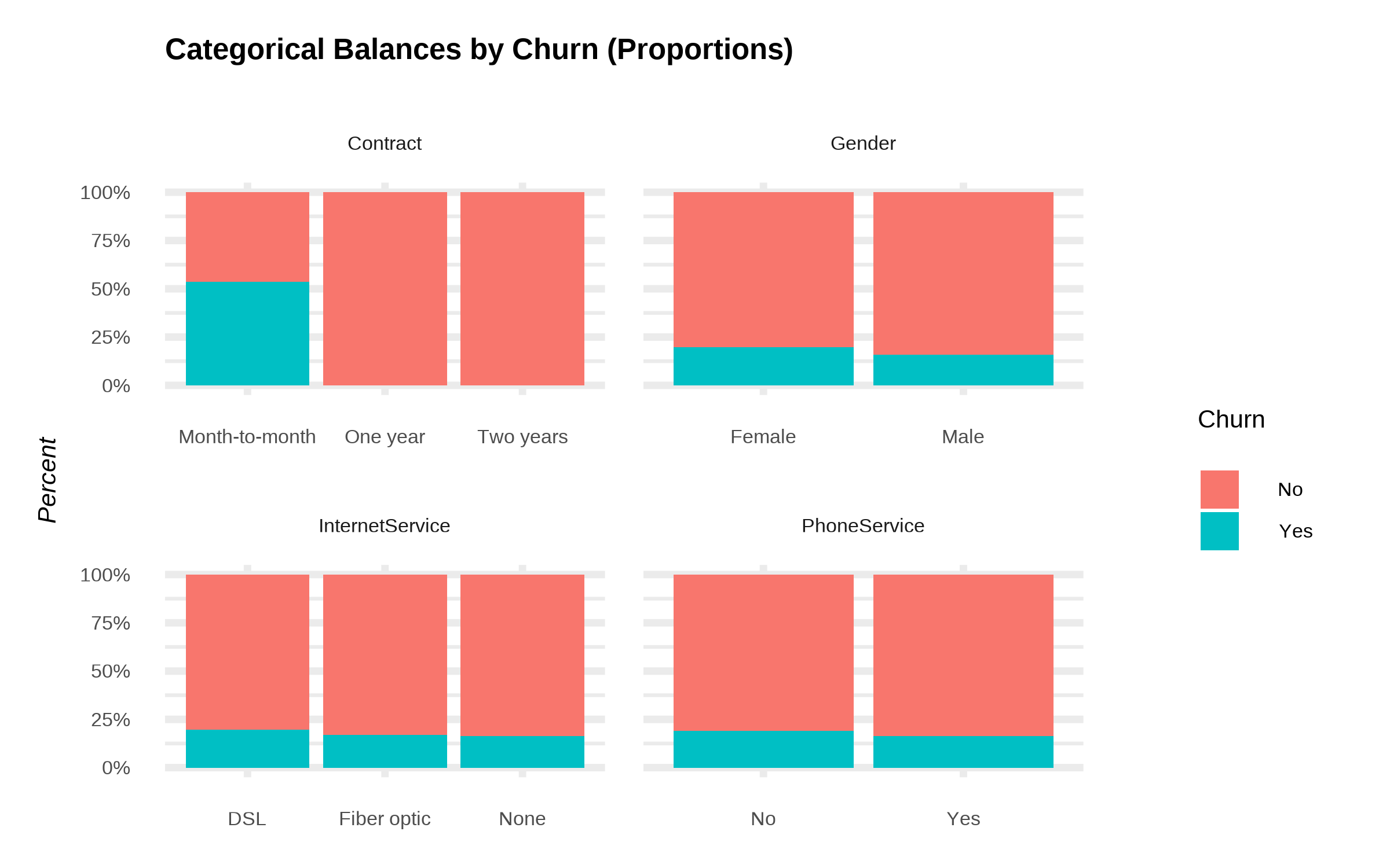
Categorical Proportions by Churn
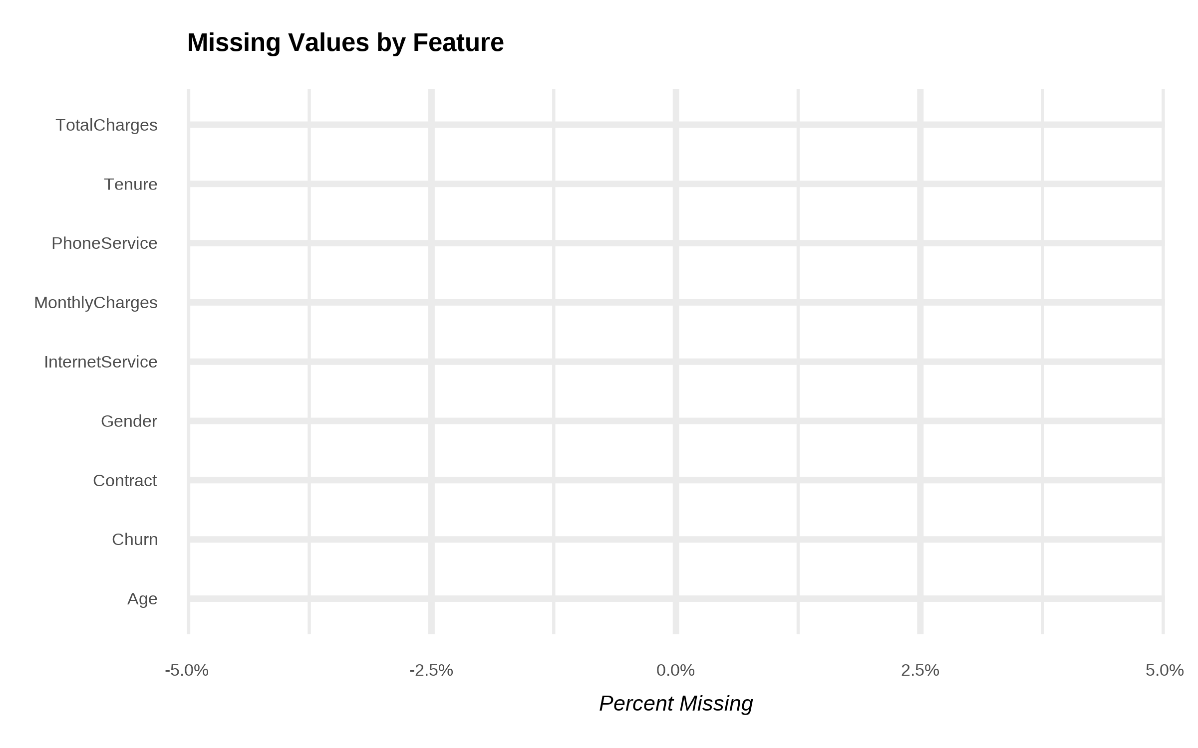
Missingness Overview
As can be seen from the following table, there is no missing data.
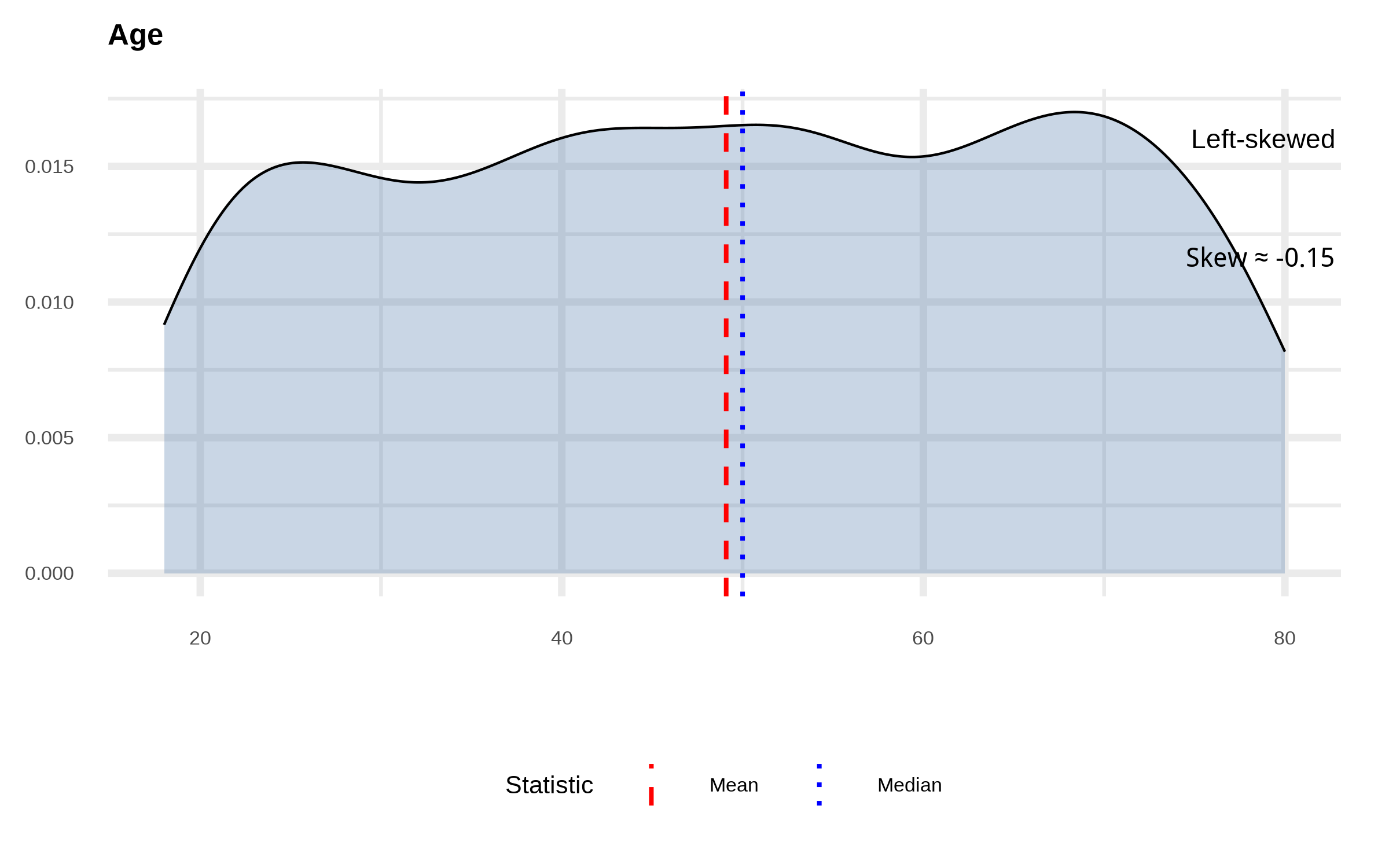
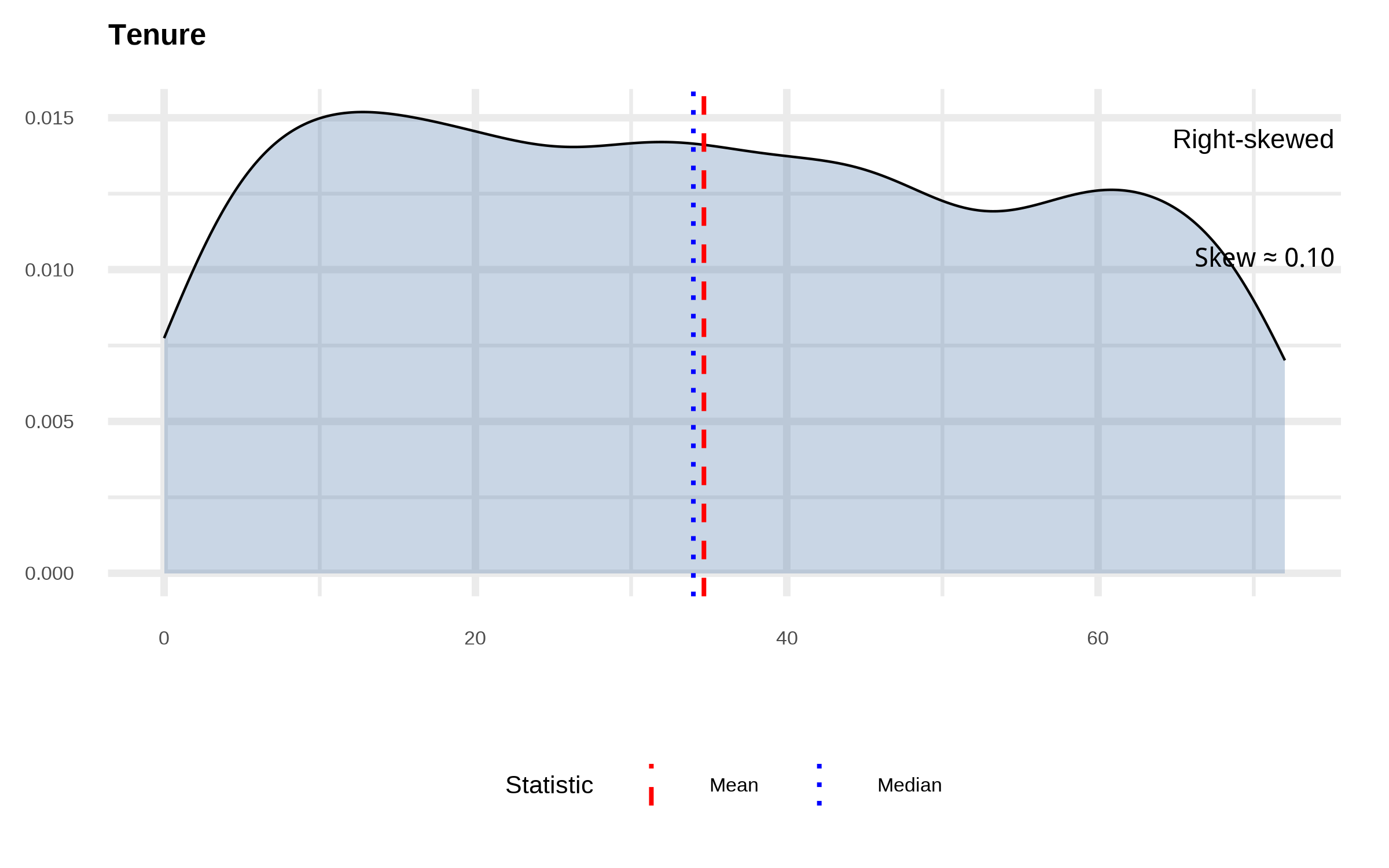
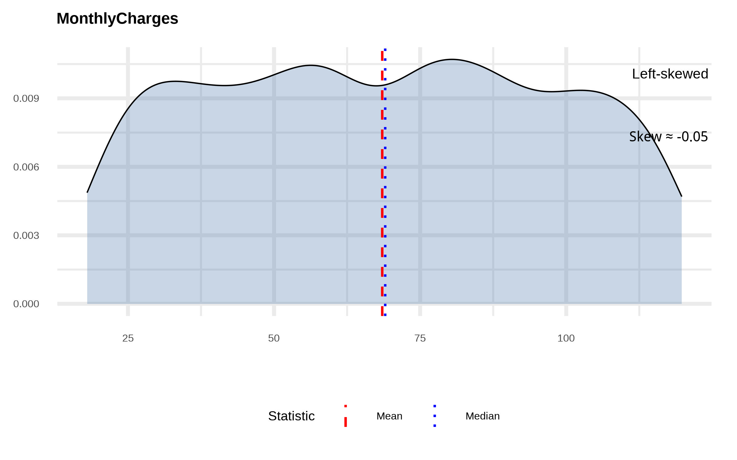
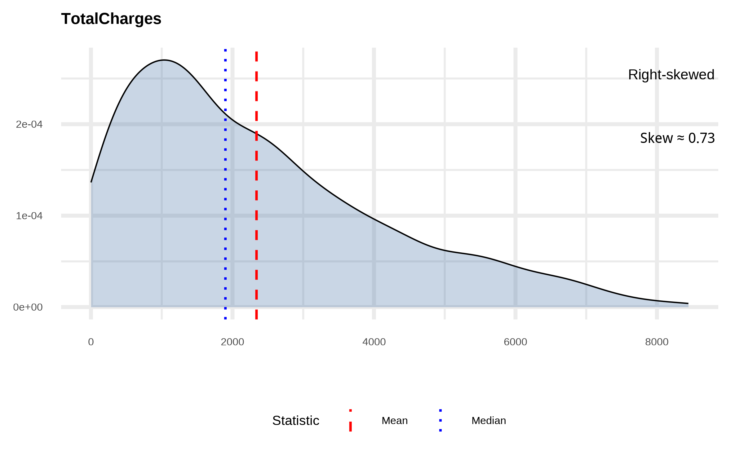
Skewness
Quick skew check (numeric)
Skewness
| TotalCharges |
1000 |
2339.68 |
1900.12 |
1808.26 |
7247.88 |
Right-skewed |
| Age |
1000 |
49.09 |
50.00 |
18.17 |
80.00 |
Left-skewed |
| Tenure |
1000 |
34.68 |
34.00 |
21.04 |
72.00 |
Right-skewed |
| MonthlyCharges |
1000 |
68.51 |
69.02 |
29.07 |
118.93 |
Left-skewed |
Skew check
The last plot suggest that most customers generate relatively low revenue, but a smaller group contributes disproportionately higher revenue. This suggest that the company may rely heavily on a minority of high-value customers.
Churn vs Non-Churn Proportions
Categorical features of interest
| Yes |
Contract |
Month-to-month |
| No |
Contract |
Two years |
| No |
Gender |
Male |
| No |
PhoneService |
Yes |
| No |
PhoneService |
No |
Stacked bar (counts by category)
Normalized bar (proportions within each category)
Bivariate (Churn vs. Features)
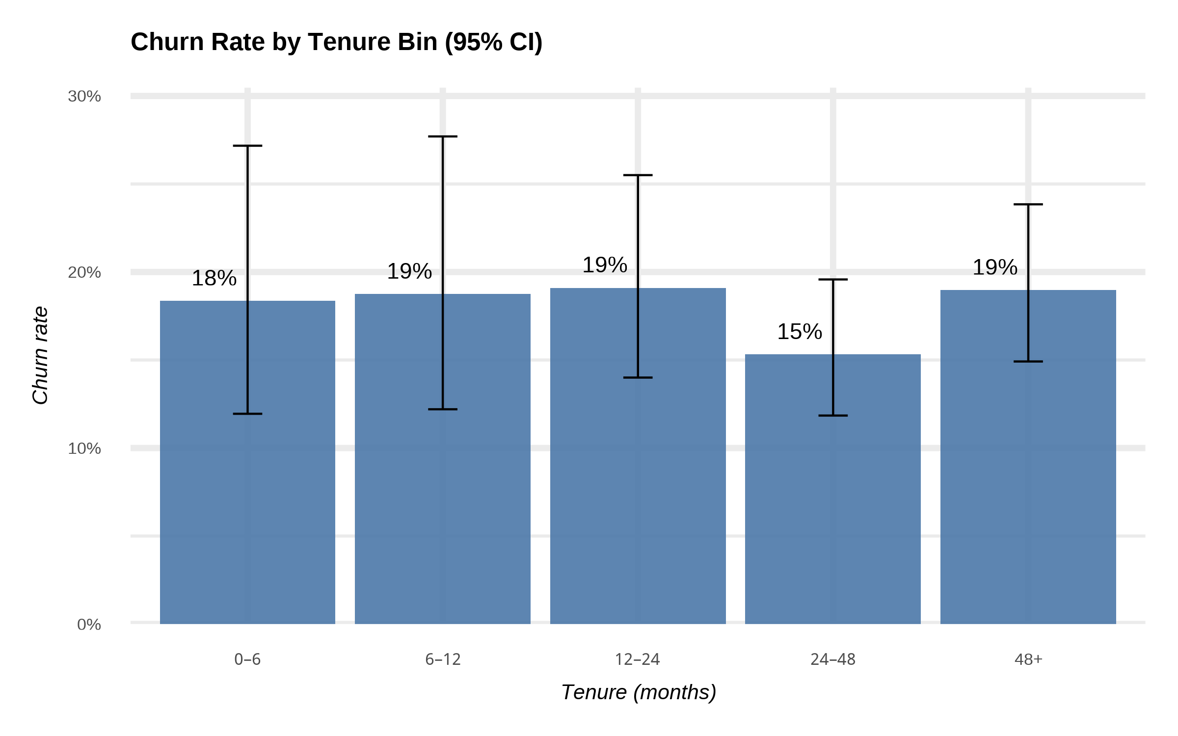
Churn rate by Tenure bins (0-6, 6-12, 12-24, 24-48, 48+)
Tenure is how long a customer has been with the company (in months). Following is the hypothesis,
Customer who are new (short tenure) are more likely to churn; customers who have stayed longer are “stickier”
To test this,
- Group customers into bins of tenure (0-6 months, 6-12, etc.).
- Compute churn rate = (# churned customers) / (total customers) in each bin.
- Plot churn rate across bins to visualize patterns.
If churn is very high in 0-6 months bin, that means the company has an onboarding / early experience problem.
Data Frame with Tenure Bin tags
| Male |
71 |
One year |
12–24 |
| Male |
26 |
Two years |
48+ |
| Female |
73 |
Two years |
48+ |
| Male |
46 |
Month-to-month |
48+ |
| Female |
37 |
Two years |
6–12 |
Tenure statistics
| 0–6 |
18 |
98 |
0.18 |
0.12 |
0.27 |
| 6–12 |
18 |
96 |
0.19 |
0.12 |
0.28 |
| 12–24 |
34 |
178 |
0.19 |
0.14 |
0.26 |
| 24–48 |
51 |
333 |
0.15 |
0.12 |
0.20 |
| 48+ |
56 |
295 |
0.19 |
0.15 |
0.24 |
Because churn rate is an estimate from data, we add 95% confidence interval using the Wilson method.
Chi-Square test
    Pearson's Chi-squared test

data:  table(df_tenure$tenure_bin, df_tenure$Churn)
X-squared = 1.9758, df = 4, p-value = 0.7402
Not significant.
Logistic regression test
Call:
glm(formula = Churn ~ tenure_bin, family = binomial, data = df_tenure)

Coefficients:
                Estimate Std. Error z value Pr(>|z|)
(Intercept)     -1.49165    0.26087  -5.718 1.08e-08 ***
tenure_bin6–12   0.02532    0.36937   0.069    0.945
tenure_bin12–24  0.04820    0.32313   0.149    0.881
tenure_bin24–48 -0.21843    0.30201  -0.723    0.470
tenure_bin48+    0.04054    0.30016   0.135    0.893
---
Signif. codes:  0 '***' 0.001 '**' 0.01 '*' 0.05 '.' 0.1 ' ' 1

(Dispersion parameter for binomial family taken to be 1)

    Null deviance: 933.63  on 999  degrees of freedom
Residual deviance: 931.61  on 995  degrees of freedom
AIC: 941.61

Number of Fisher Scoring iterations: 4
Only the Intercept is statistically significant. So, we can’t accept out hypothesis.
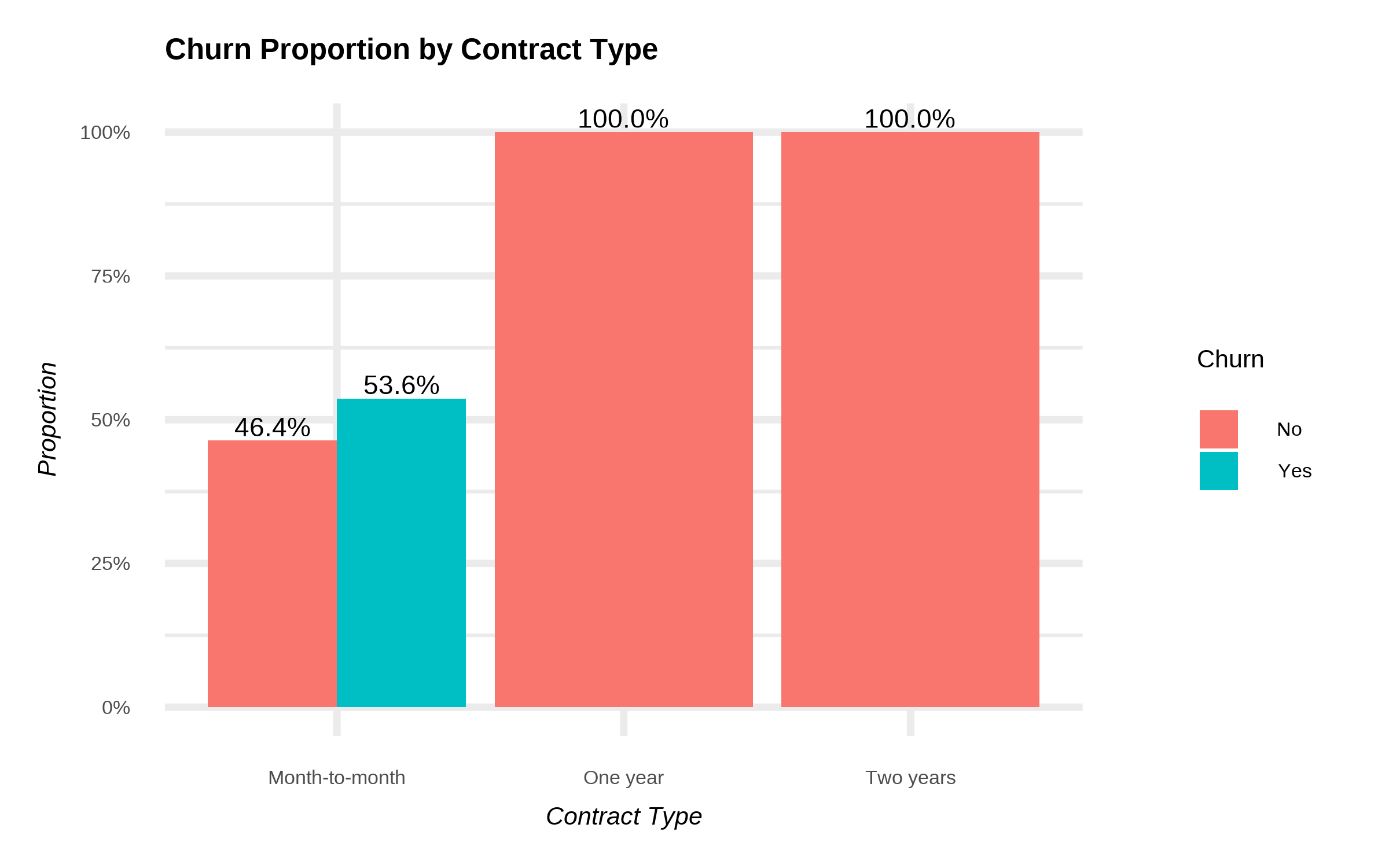
Contract Type vs. Churn
Goal: Show how churn differs by contract type.
Hypothesis: Month-to-month has higher churn than One/Two year contracts.
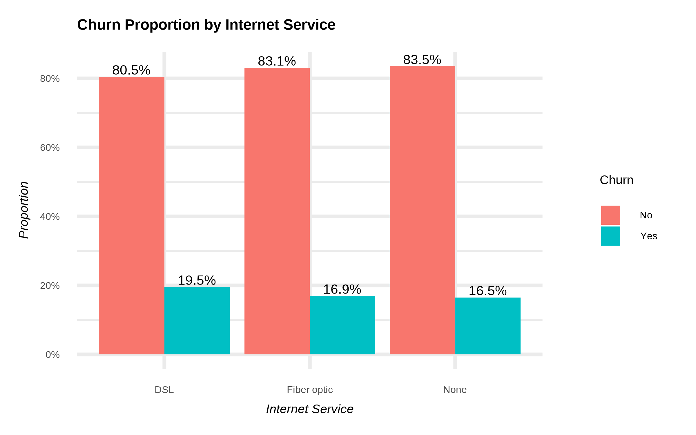
Internet Service vs. Churn
Goal: Compare churn across DSL / Fiber optic / No Internet.
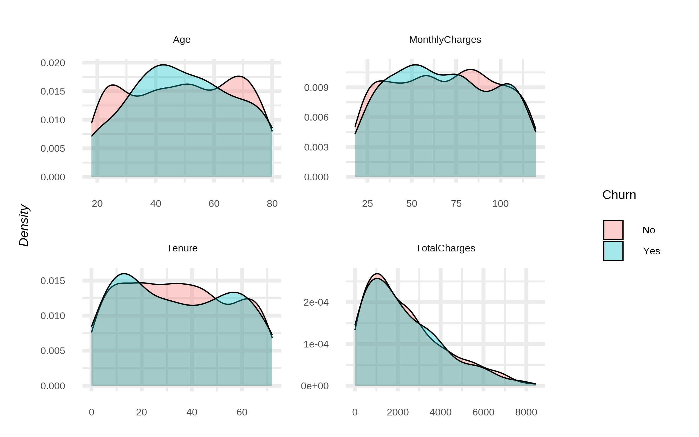
Numeric Densities by Churn
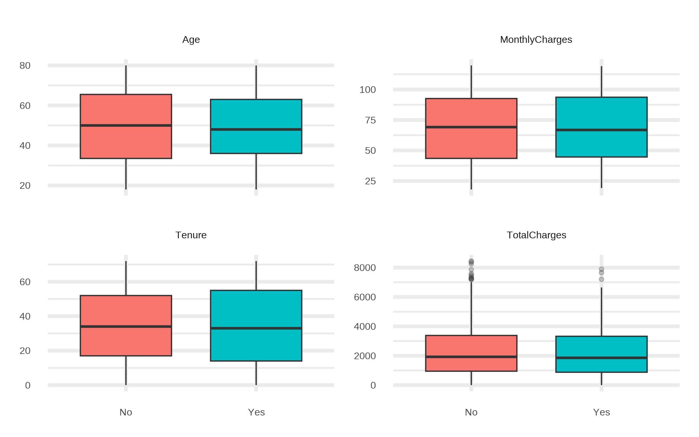
Numeric Box Plots by Churn
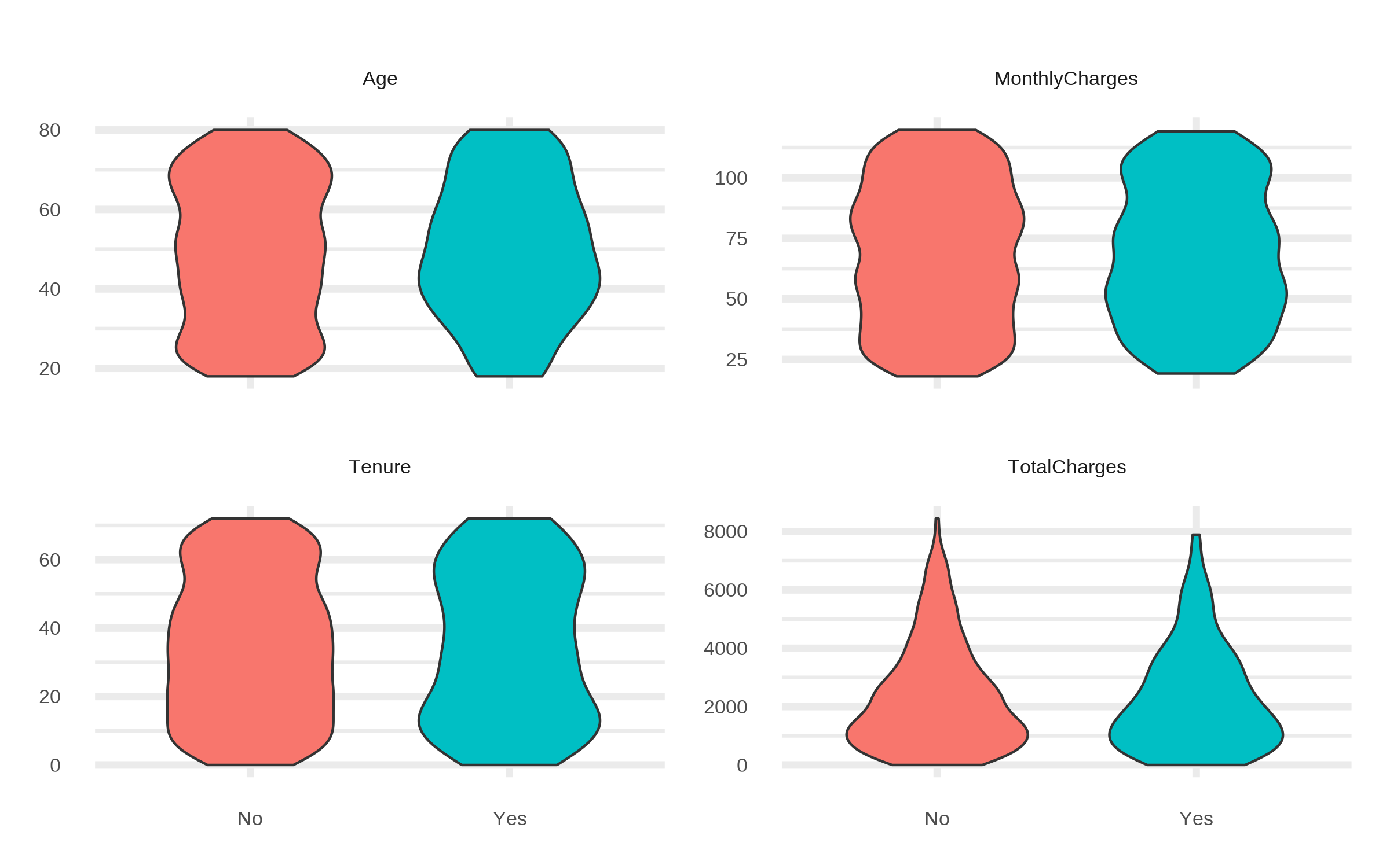
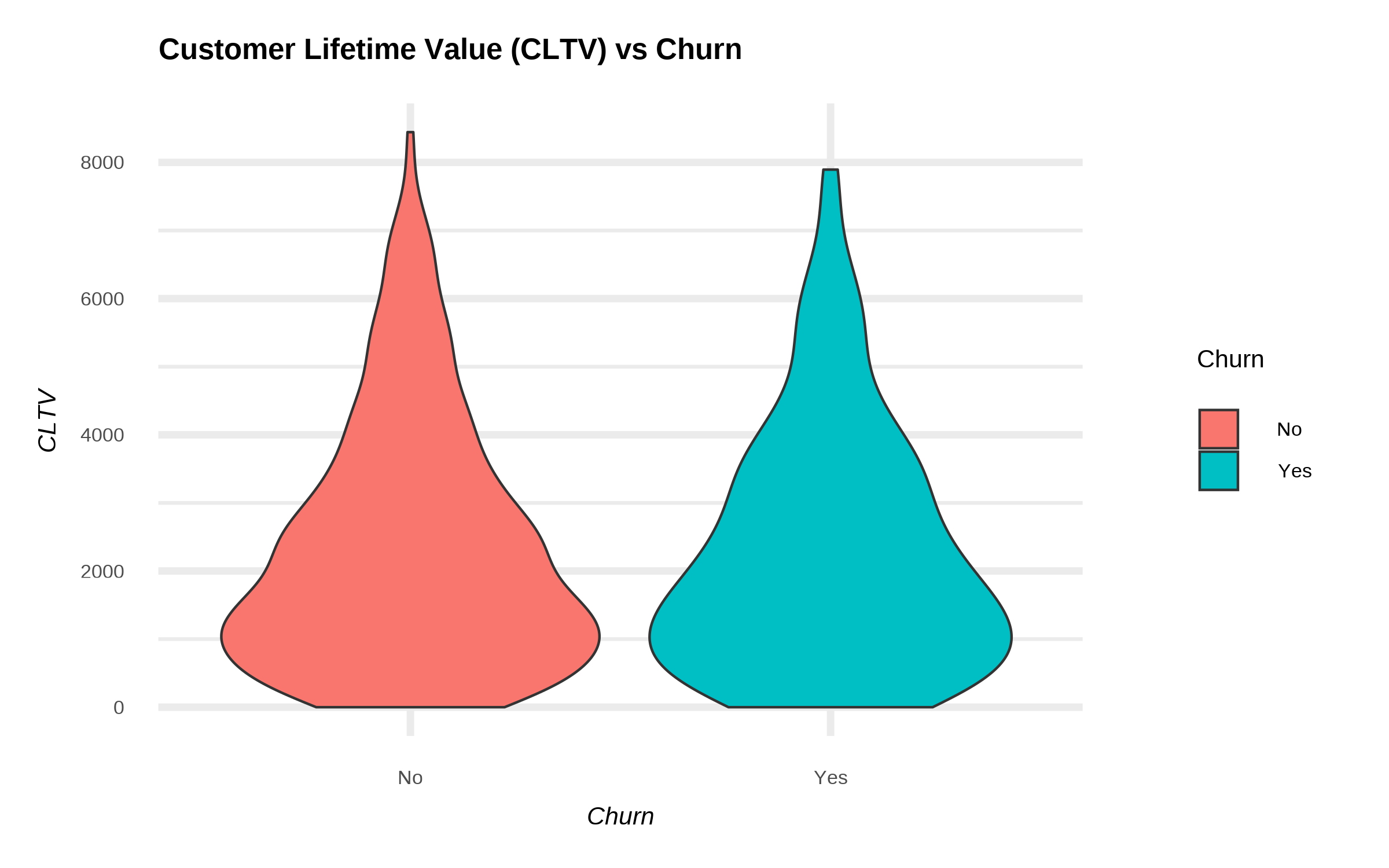
Numeric Violin Plots by Churn
Multivariate Relationships
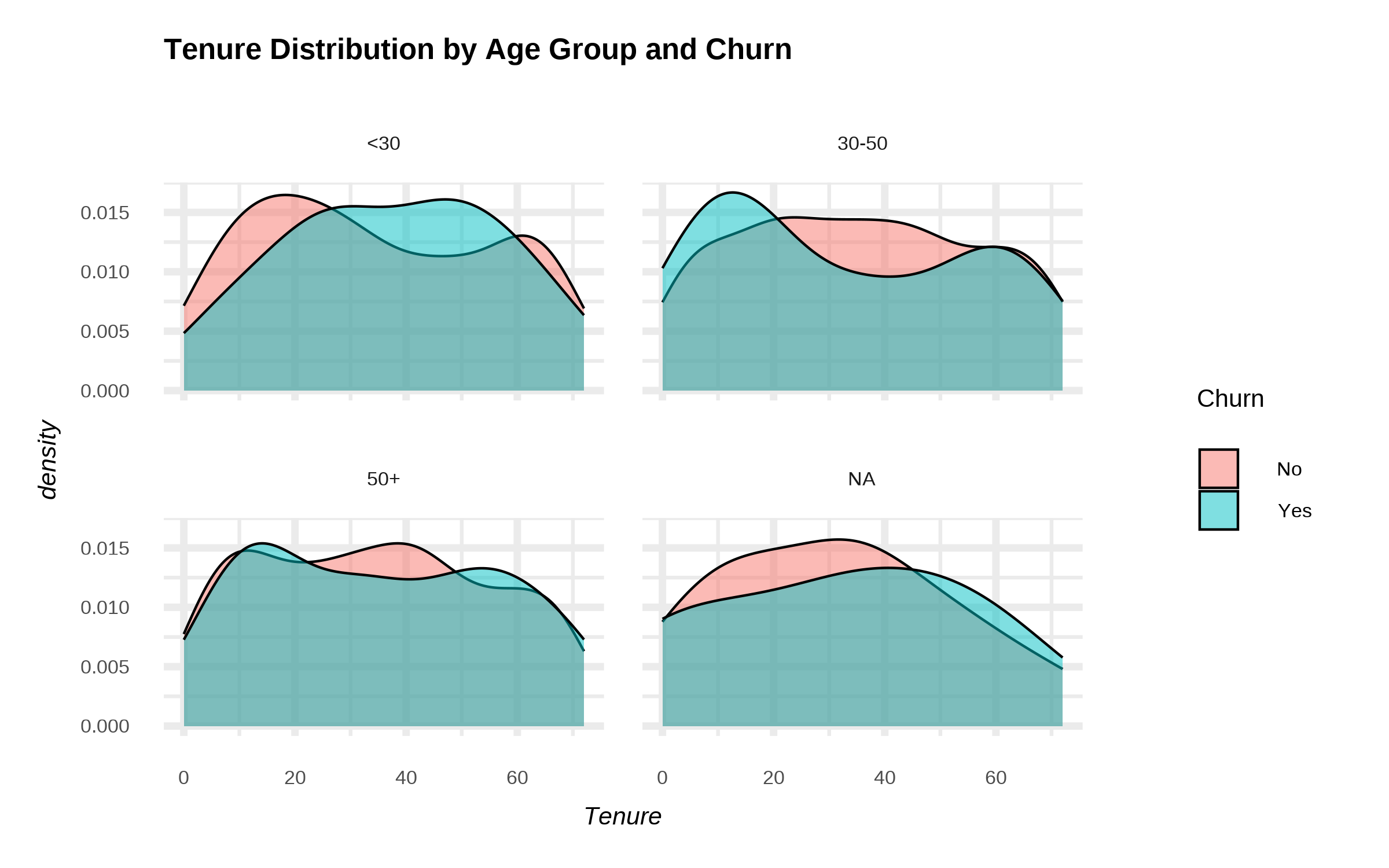
Age x Tenure x Churn
Data for `Tenure Distribution by Age Group and Churn'
| Male |
48 |
6 |
Yes |
None |
One year |
60.76 |
364.56 |
No |
30-50 |
| Male |
74 |
13 |
Yes |
DSL |
One year |
100.15 |
1301.95 |
No |
50+ |
| Female |
74 |
46 |
Yes |
DSL |
Month-to-month |
73.52 |
3381.92 |
Yes |
50+ |
| Male |
24 |
2 |
Yes |
None |
One year |
22.97 |
45.94 |
No |
<30 |
| Male |
28 |
4 |
No |
None |
Two years |
35.16 |
140.64 |
No |
<30 |
Following plot shows distributions of Tenure across age groups and split by Churn,
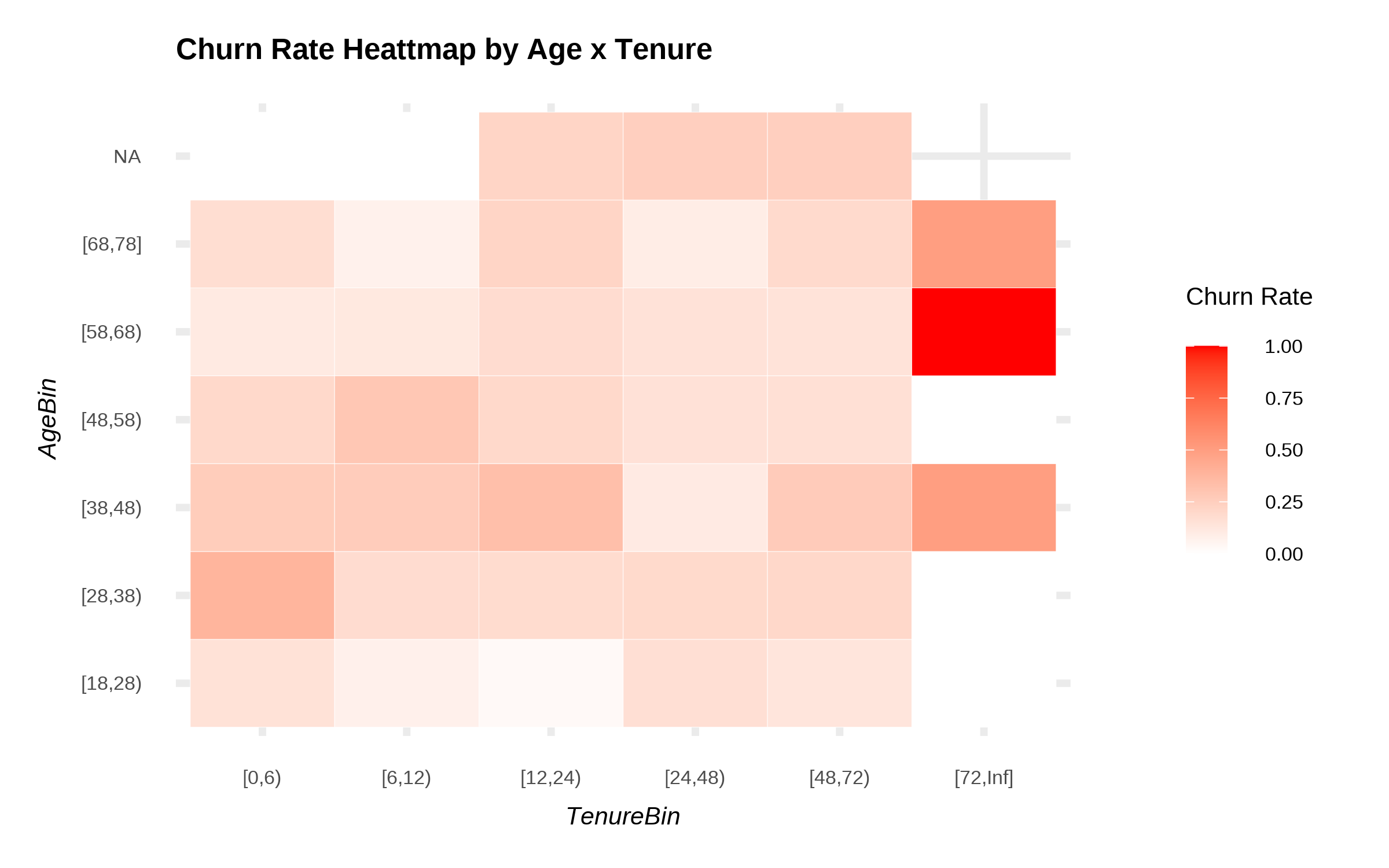
For extra clarity, following is a Heatmap,
| [68,78] |
[72,Inf] |
0.50 |
| [18,28) |
[48,72) |
0.13 |
| [38,48) |
[48,72) |
0.27 |
| [58,68) |
[72,Inf] |
1.00 |
| [18,28) |
[12,24) |
0.03 |
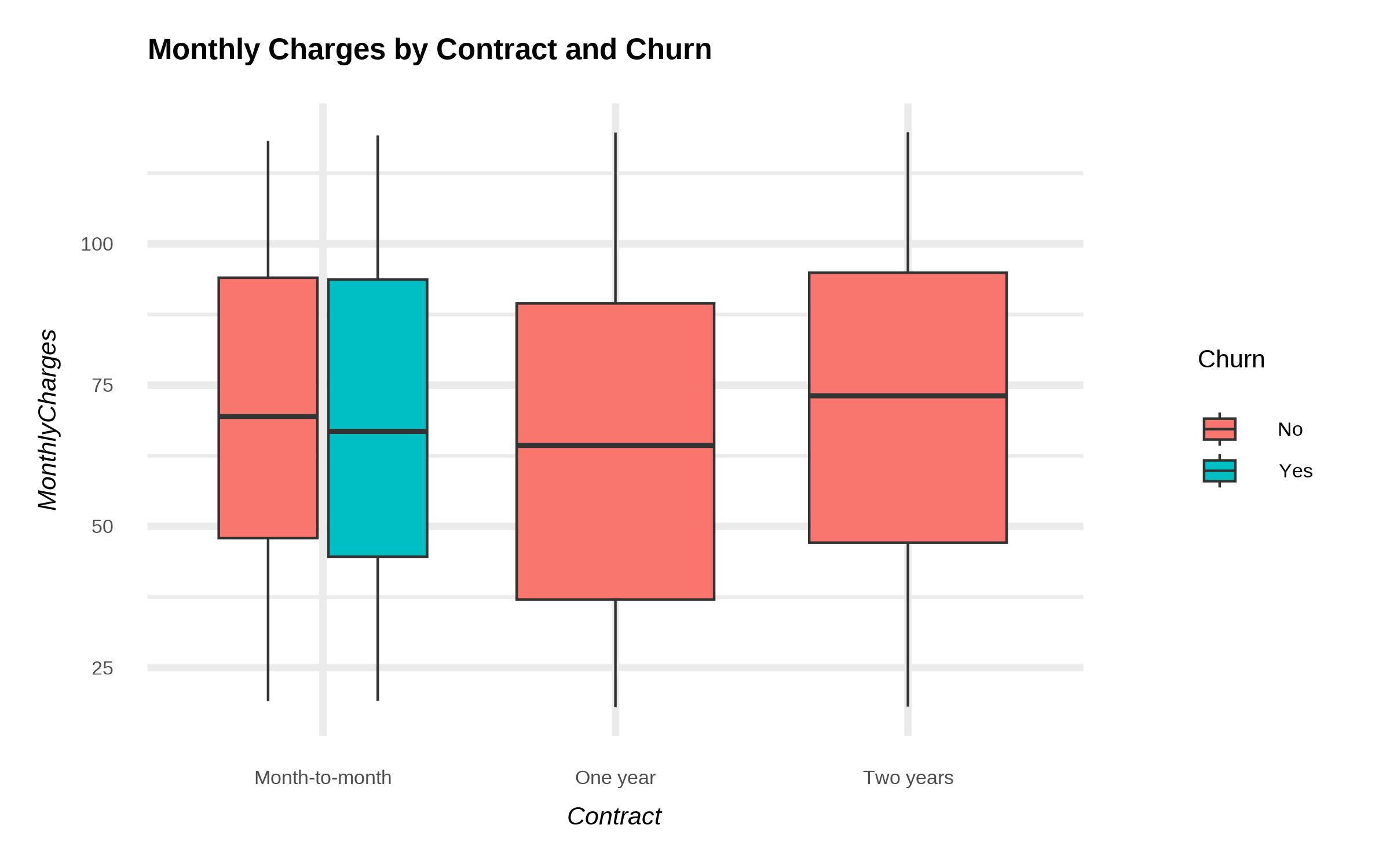
MonthlyCharges x Contract x Churn
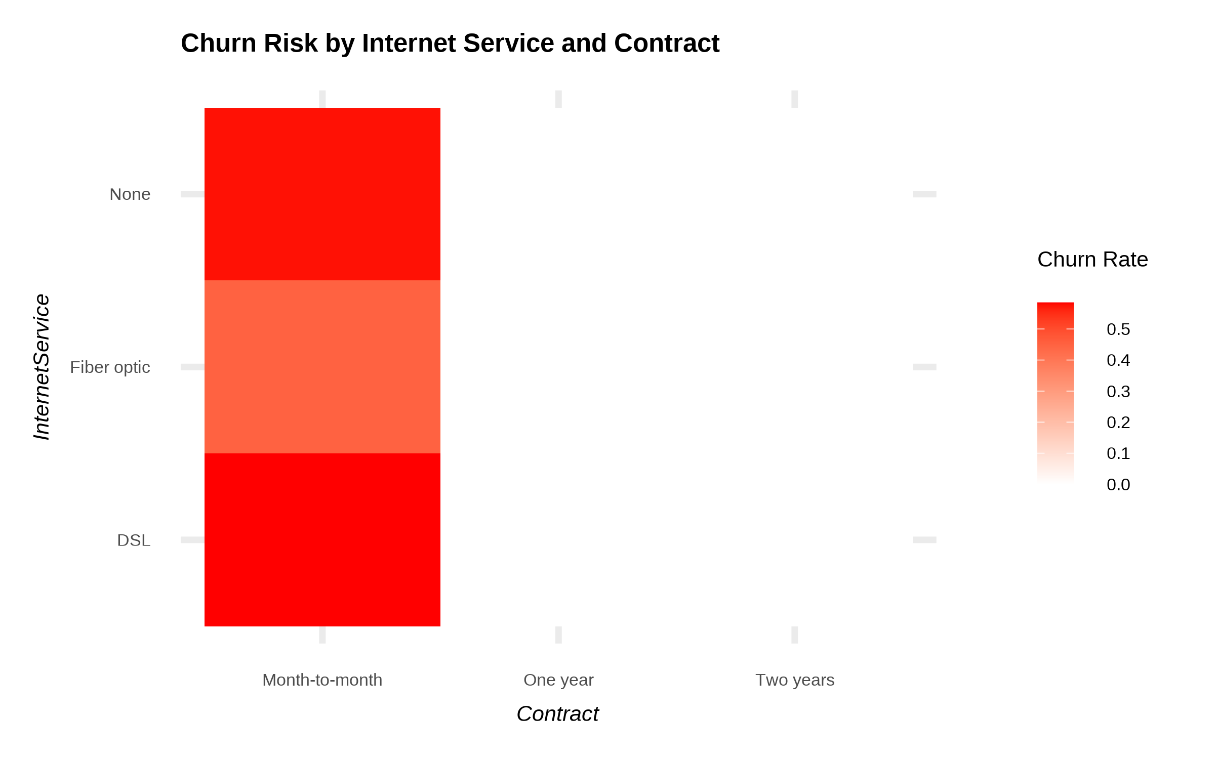
InternetService x Contract (churn risk heatmap)
Feature Engineering for EDA
Customer lifetime value proxy
| Male |
25 |
30 |
Yes |
None |
Month-to-month |
41.60 |
1248.00 |
Yes |
1248.00 |
| Female |
72 |
29 |
Yes |
None |
Two years |
33.94 |
984.26 |
No |
984.26 |
| Male |
71 |
44 |
No |
Fiber optic |
Month-to-month |
107.69 |
4738.36 |
No |
4738.36 |
| Male |
62 |
55 |
Yes |
DSL |
Two years |
73.99 |
4069.45 |
No |
4069.45 |
| Female |
40 |
4 |
Yes |
DSL |
Two years |
119.24 |
476.96 |
No |
476.96 |
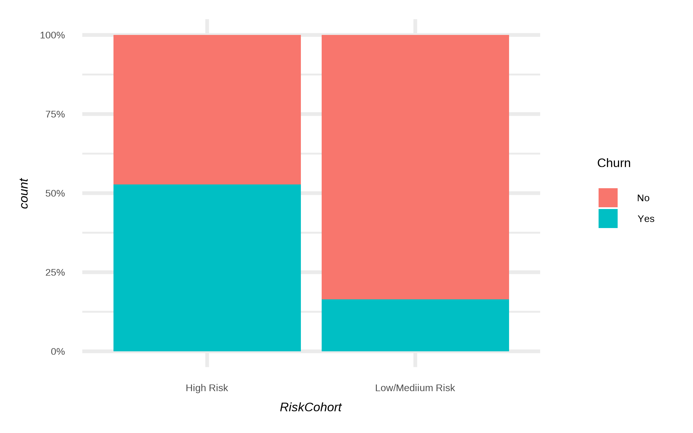
At-risk cohorts (cohort flagging)
Create a derived feature for risk segments,
Risk Cohort table
| Male |
79 |
37 |
Yes |
Fiber optic |
One year |
26.29 |
972.73 |
No |
Low/Mediium Risk |
| Male |
49 |
4 |
Yes |
DSL |
Two years |
35.33 |
141.32 |
No |
Low/Mediium Risk |
| Female |
80 |
28 |
Yes |
Fiber optic |
Month-to-month |
109.59 |
3068.52 |
Yes |
Low/Mediium Risk |
| Male |
21 |
21 |
No |
None |
Month-to-month |
61.76 |
1296.96 |
No |
Low/Mediium Risk |
| Male |
35 |
34 |
No |
DSL |
Month-to-month |
93.71 |
3186.14 |
Yes |
Low/Mediium Risk |
High-risk customers churn much more, with over half leaving. Low/medium-risk customers mostly stay, with only a small fraction churning. This highlights the value of risk segmentation: high-risk cohorts require targeted retention strategies to reduce churn and improve overall customer retention.
Correlation & Association
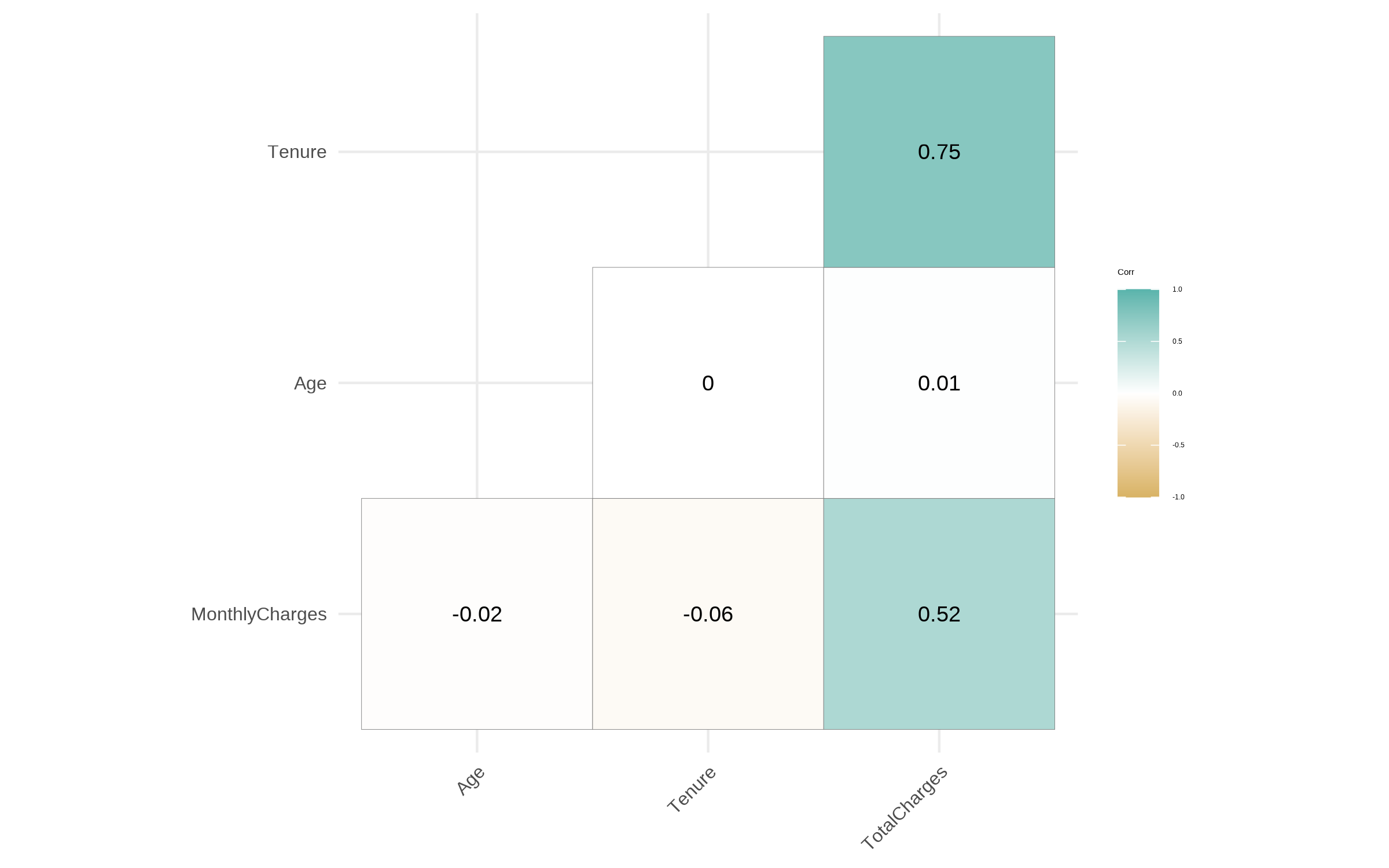
Numeric-only correlation matrix
Chi-square + Cramer’s V for categorical vs. Churn
Cramér’s V - Effect size measure
| Contract |
436.65 |
2 |
0.00 |
0.66 |
| Gender |
2.34 |
1 |
0.13 |
0.05 |
| PhoneService |
0.88 |
1 |
0.35 |
0.03 |
| InternetService |
1.30 |
2 |
0.52 |
0.04 |
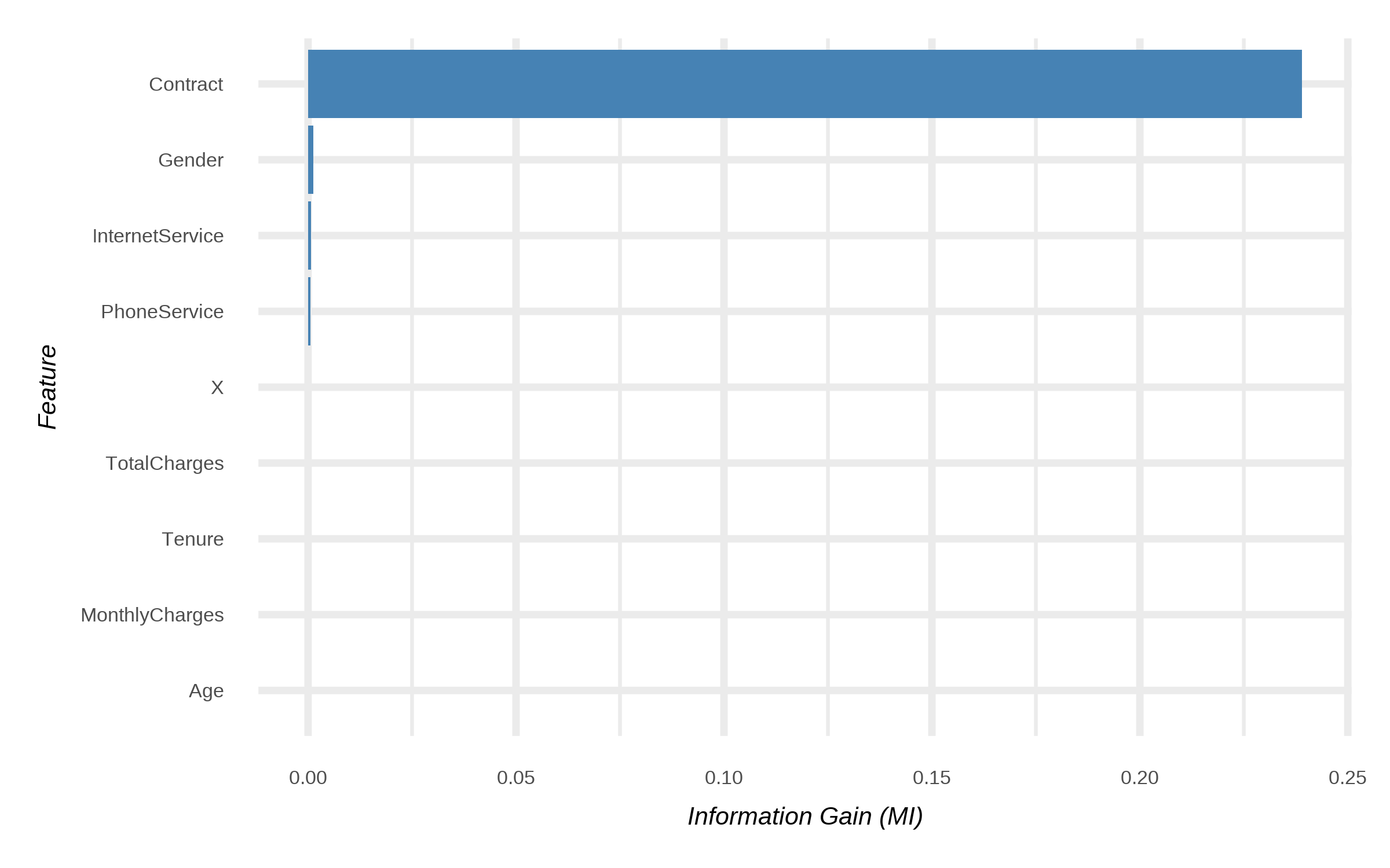
Which shows that, to predict churn, Contract is a strong (because of low p_value) predictor. Next up are, Gender, PhoneService, and InternetService.
Survival-style Analysis
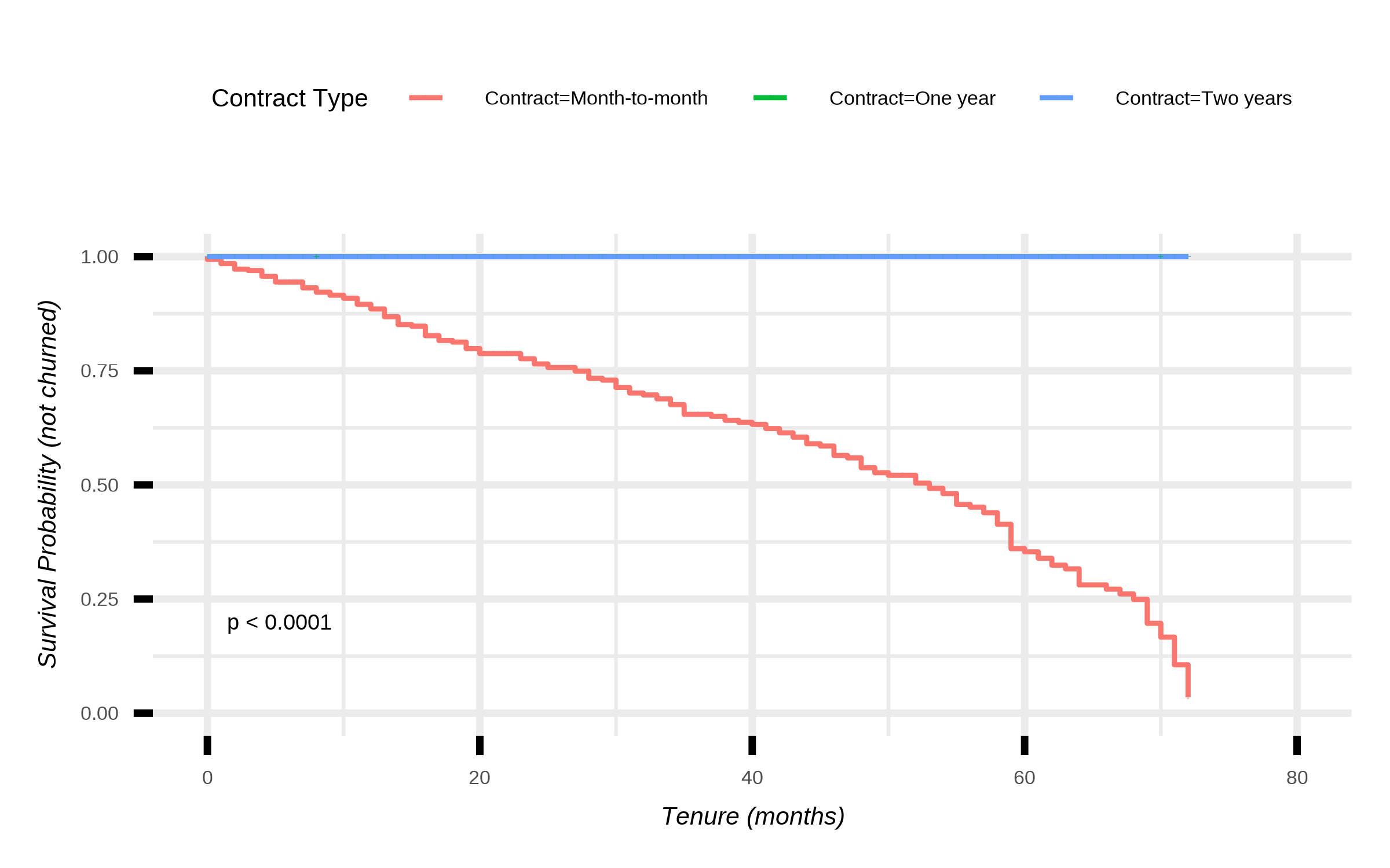
The Kaplan-Meier estimator generates the survival curves for different contract types. It answers the following simple yet important question,
What percentage of customers are still active after X months, depending on their contract type?
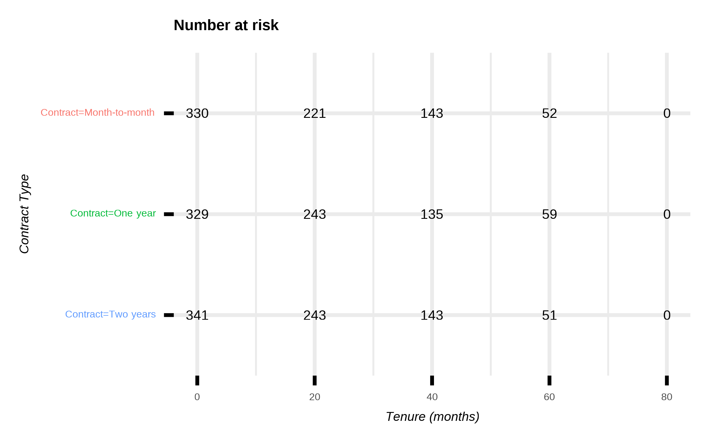
The Kaplan–Meier survival curves show how long customers remain active without churning, based on contract type. Month-to-month customers (red) churn steadily, with survival probability dropping below 50% by around 40–50 months. In contrast, one-year (green) and two-year contracts (blue) maintain nearly perfect retention over time, with very little churn observed. The p-value (<0.0001) indicates these differences are highly statistically significant. In short, customers on longer-term contracts are far less likely to churn, while month-to-month customers have much higher and earlier churn rates. Contract length is thus a critical factor in customer retention.
Feature Importance
Logistic Regression for Feature Importance
Logistic model estimates
| GenderMale |
-0.54 |
0.29 |
-1.88 |
0.06 |
| (Intercept) |
1.56 |
0.97 |
1.62 |
0.11 |
| InternetServiceFiber optic |
-0.55 |
0.35 |
-1.60 |
0.11 |
| InternetServiceNone |
-0.41 |
0.34 |
-1.21 |
0.23 |
| MonthlyCharges |
-0.01 |
0.01 |
-1.12 |
0.26 |
| TotalCharges |
0.00 |
0.00 |
0.80 |
0.42 |
| PhoneServiceYes |
-0.15 |
0.28 |
-0.54 |
0.59 |
| Tenure |
-0.01 |
0.02 |
-0.38 |
0.71 |
| Age |
0.00 |
0.01 |
-0.30 |
0.76 |
| ContractOne year |
-20.84 |
1121.38 |
-0.02 |
0.99 |
The above table is sorted with respect to p-value. The only significant feature for predicting Churn according to this model is InternetServiceFiber optic. Even though, PhoneService and the intercept has a low p-value, they are not significant.
Random Forest for Feature Importance
Random forest estimates
| Contract |
39.05 |
51.17 |
51.44 |
83.57 |
| TotalCharges |
3.78 |
-4.51 |
1.18 |
23.13 |
| MonthlyCharges |
0.66 |
-1.74 |
-0.59 |
23.07 |
| Age |
1.86 |
2.24 |
2.86 |
21.91 |
| Tenure |
3.90 |
-2.09 |
2.14 |
20.05 |
| InternetService |
-1.72 |
1.23 |
-0.36 |
6.38 |
| Gender |
1.19 |
-0.32 |
0.63 |
3.81 |
| PhoneService |
-0.23 |
1.18 |
0.72 |
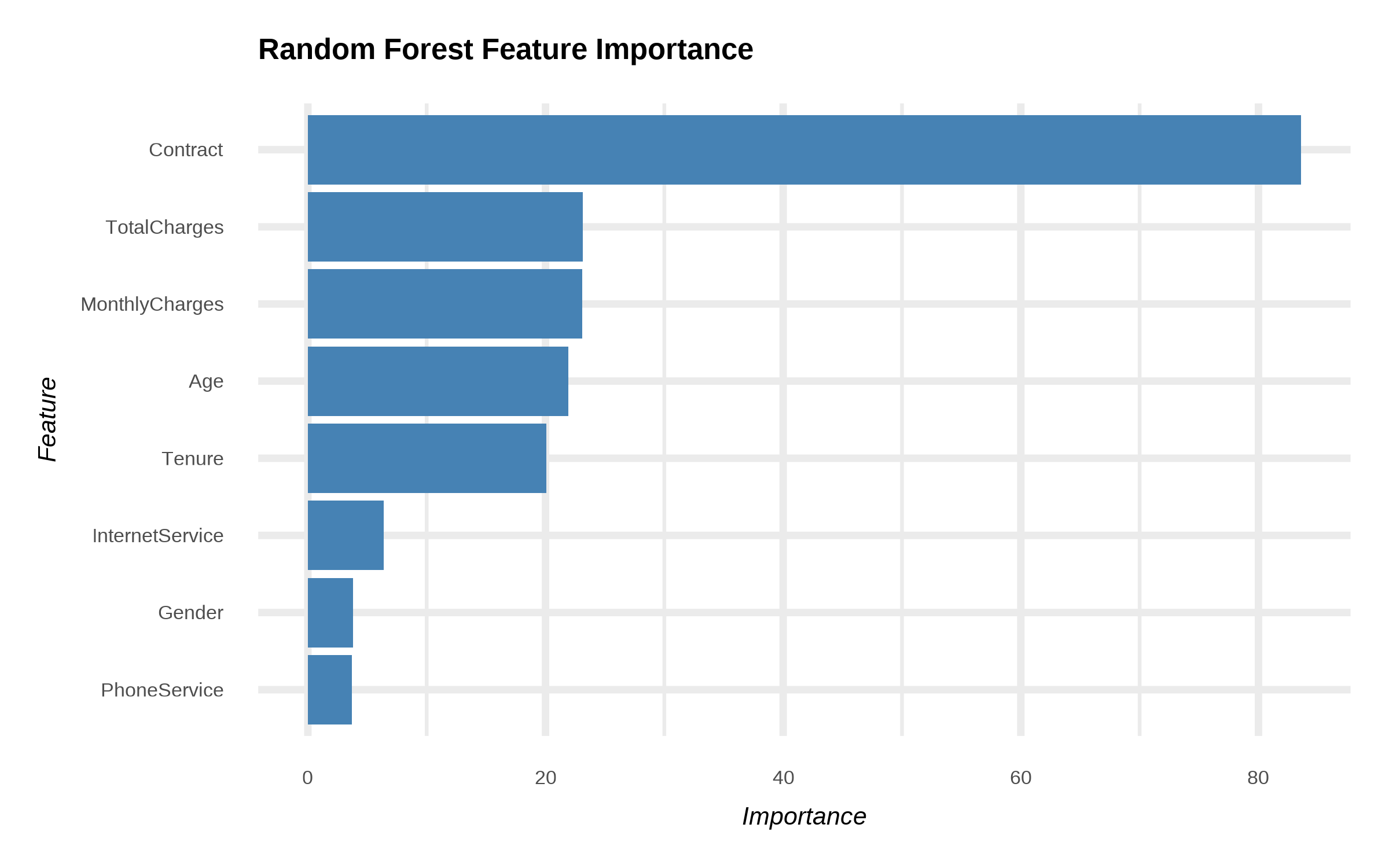
3.72 |
The random forest importance table shows that Contract is the most influential predictor of churn, with the highest values in both MeanDecreaseAccuracy (44.71) and MeanDecreaseGini (79.11). MonthlyCharges, Age, TotalCharges, and Tenure also contribute meaningfully, though at lower levels, indicating that financial and tenure-related variables affect churn risk. InternetService, Gender, and PhoneService have much smaller importance scores, suggesting they add little predictive value. Overall, contract type dominates as the key driver, followed by monetary and tenure factors, while demographic or service-type variables play a minor role in predicting churn.